“Cloud” visualizations, or “tag clouds” are great ways of summarizing a bunch of data when a frequency table or list would be too unwieldy or confusing. They’re most commonly encountered in the context of text mining but we could really use them with anything where there’s a large number of categories or bins. In the most common version of these visualizations, the size of category or bin name (or word, in the case of word clouds) is indicative of its frequency. Here’s an example using the text of a favorite poem of mine, The Love Song of J. Alfred Prufrock by T.S. Eliot (made using a free, online word cloud generator available here).

In the last post about this project, we clustered genes that we identified as differentially-expressed in dementia in samples from a region of the brain critical for memory formation (the hippocampus) using the \(k\)-medoids partitioning method. We also discussed gene ontologies, or terms that tell us about where gene products are found in cells, what they do, and which “big picture” biological processes they participate in. I introduced you to the mygene package for R that has query functions for an open-source database of gene ontology information. We used it to take a peak at what the medoids we identified (and want to use as new features for models of dementia risk) do and where they might be found in cells.

In this post, we’ll make some “term clouds” using the wordcloud package for R to help crack open the three clusters we made for hippocampus dementia-associated genes. Genes that participate in the same or related biological processes tend to have similar expression patterns and may cluster together. We’ll use term clouds to get a sense of whether or not this is the case for the three clusters of genes from hippocampal samples that we found to potentially be involved in dementia. Maybe there are different processes represented in the different clusters. We’ll find out!

On tap for this post:

1. Load Libraries & Data - If you’re running the Jupyter notebook copy of this post from within a cloned copy of the project repo on GitHub, you have everything you need to make this work. Alternatively, you can download the files directly from the repo data folder and modify the code to read the .Rds files from the folder you put them in. All this code was written using an Anaconda distribution of R version 3.4.1.

2. \(k\)-medoid Cluster Assignments - We’ll run the CLARA algorithm and grab lists of the genes in each cluster.

3. Query mygene.info For Biological Process Terms - We’ll make lists of the terms associated with the genes in each cluster.

4. Term Clouds - We’ll look at the biological processes associated with the genes in each cluster.

Let’s get started!

Load Libraries & Data

First, let’s get some libraries loaded.

library(cluster)        # k-medoids via CLARA
library(mygene)         # To query mygene.info for biological process terms
library(wordcloud)      # For clouds of annotation terms/words

Now, we’ll read in the data. This includes the normalized tables of gene expression levels (in fragments per kilobase million, or FPKM), some information about the samples (including which ones come from the hippocampus), and lists of the differentially-expressed-in-dementia genes we identified for each of the four brain regions in the dataset.

# load normalized FPKM values, sample info, DE gene lists for brain regions, annotations
fpkm_table <- readRDS(file='data/normalized_fpkm_matrix.Rds')
sample_info <- readRDS(file='data/sample_info.Rds')
brain_reg_sig_genes <- readRDS(file='data/brain_reg_sig_genes.Rds')

# make FPKM numeric matrix
fpkm_mat <- as.matrix(fpkm_table)
class(fpkm_mat) <- 'numeric'

# standardize
fpkm_standard_mat <- t(scale(t(fpkm_mat)))

# pull out individual brain region DE gene list
hip_genes <- brain_reg_sig_genes$hip_genes

# subset FPKM matrix to just HIP samples and HIP DE genes
hip_samples <- sample_info$rnaseq_profile_id[which(sample_info$structure_acronym == 'HIP')]
hip_data <- fpkm_standard_mat[hip_genes, colnames(fpkm_standard_mat) %in% hip_samples]

\(k\)-medoid Cluster Assignments

CLARA is an algorithm for doing \(k\)-medoids clustering. We’ll instruct the clara() method to find \(k=3\) clusters for the 277 differentially-expressed genes we found in hippocampus samples.

# set an RNG seed for reproducibility
set.seed(424)

# run CLARA on HIP FPKM values
hip_final_clara <- clara(hip_data, k=3, metric = 'euclidean',
                         samples=1000, sampsize=250, pamLike=TRUE)

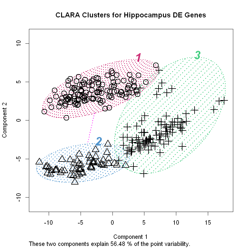
Here’s a plot of the data along the first two principal components, which allows us to visualize the clusters.

clusplot(hip_final_clara, color=TRUE, shade=TRUE,
         labels=4, col.txt='black', col.p='black',
         col.clus=c('seagreen3', 'steelblue3', 'violetred3', 'sienna3'),
         cex=2, main = 'CLARA Clusters for Hippocampus DE Genes',
         ylim=c(-11,11), lwd=2, lty=3)

The clara object contains many useful things.

names(hip_final_clara)

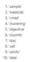
In the last post, we accessed the medoids attribute to make new variables for models of dementia risk. This time, we’ll get the cluster assignments for each gene from the clustering attribute. The row names for our original dataframe (and thus for everything from the clara object) are Entrez Gene numbers that are unique identifiers of the genes. To get lists of the genes in each cluster, we’ll simply get the row names that are associated with the different cluster assignments using which().

# create cluster assignment dataframe
hip_clusters <- data.frame(cluster_assignment=hip_final_clara$clustering)

# list of genes in each cluster
hip_genes01 <- rownames(hip_clusters)[which(hip_clusters$cluster_assignment == 1)]
hip_genes02 <- rownames(hip_clusters)[which(hip_clusters$cluster_assignment == 2)]
hip_genes03 <- rownames(hip_clusters)[which(hip_clusters$cluster_assignment == 3)]

Query the mygene.info Database for Biological Process Terms

The queryMany() method from the mygene package let’s look up many genes at one time. We set the scopes argument equal to whatever it is we’re looking the genes up by, which in our case is the Entrez Gene ID number. We’ll tell it to return the gene ontologies (GO).

# query mygene.info
hip_query01 <- queryMany(hip_genes01, scopes='entrezgene', fields='go', species='human')
hip_query02 <- queryMany(hip_genes02, scopes='entrezgene', fields='go', species='human')
hip_query03 <- queryMany(hip_genes03, scopes='entrezgene', fields='go', species='human')

The mygene.info database is a “noSQL” ElasticSearch database where each gene has a file (in JSON format) full of information. When you query this database with R, the default result is a dataframe containing nested lists (in Python, these would be nested dictionaries).

head(hip_query01)

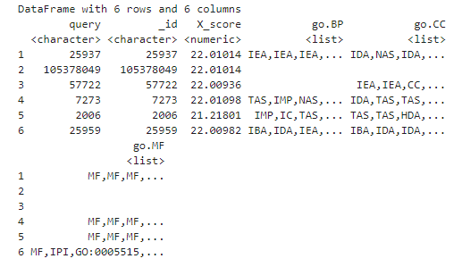
The last three columns of the query dataframe contain lists of biological process (BP), cellular component (CC), and molecular function (MF) information for each gene. A single gene can take part in many biological processes, for example. Let’s take a look at part of the BP dataframe for the first gene in the first cluster.

head(hip_query01[1, 'go.BP'][[1]])

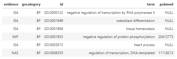
This not only provides us with the name of the biological process (term) but also with information about how it was determined to participate in that process (encoded in evidence) and the peer-reviewed publications (if any) in the scientific literature (pubmed) where we can read about the experiments providing that evidence.

The following one-liners pull out the BP terms for each gene and generate one long list of terms for each of the three clusters. Let’s break these down:

• First, we use lapply() to extract the single term columns from inside each gene’s record we pulled from the database.
• Next, we unlist() the list of term columns to concatenate them into a single list of terms.
• Finally, we wrap the entire thing in a data.frame() and set the column name as bp_terms.

# biological process (BP) gene ontology terms for each cluster
hip_cluster01_bp_terms <- data.frame(bp_terms=unlist(lapply(hip_query01$go.BP, function(x) x$term)))
hip_cluster02_bp_terms <- data.frame(bp_terms=unlist(lapply(hip_query02$go.BP, function(x) x$term)))
hip_cluster03_bp_terms <- data.frame(bp_terms=unlist(lapply(hip_query03$go.BP, function(x) x$term)))

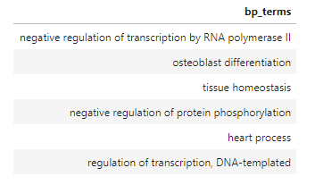
Let’s a have quick look at the first few terms for cluster #1.

head(hip_cluster01_bp_terms)

Term Clouds

We’re almost ready to make our cloud visualizations but, first, we need to get the frequencies for each of the terms. We’ll do that using table().

# make tables of BP terms for each cluster
hip_terms01_table <- table(hip_cluster01_bp_terms$bp_terms)
hip_terms02_table <- table(hip_cluster02_bp_terms$bp_terms)
hip_terms03_table <- table(hip_cluster03_bp_terms$bp_terms)

In constructing our term clouds, we’ll tell wordcloud() to use the names of the categories in the table as the “words” and the values inside as the frequencies. The wordcloud package let’s us customize a wide variety of settings. For the first cluster, we’ll tell it to plot 75 terms (max.words) with at least 2 copies in the list (min.freq). Along with the size of the words, we can also indicate how many of each term there is by color. In the examples below, the most frequent terms in the cluster are red, followed by blue and then black.

Here’s the cloud for the BP terms associated with hippocampus gene cluster #1.

set.seed(412)

# BP "term cloud" for cluster #1...
wordcloud(names(hip_terms01_table), as.numeric(hip_terms01_table),
          scale=c(1.1, .6), min.freq=2, max.words=75, random.order=T,
          rot.per=.25, colors=c('black', 'blue3', 'red3'),
          vfont=c('sans serif','plain'))

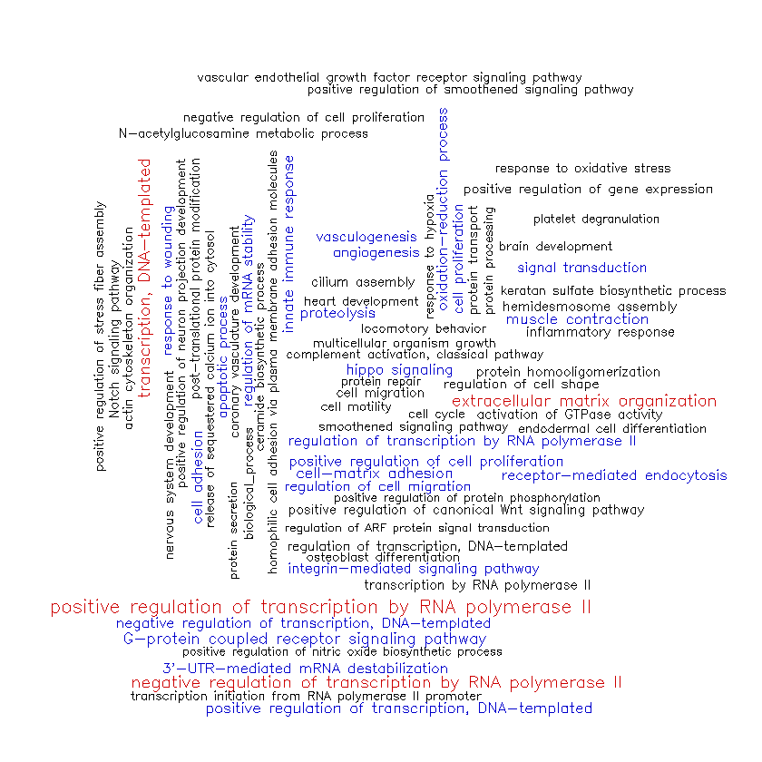
The genes in cluster #1 appear to be most strongly associated with the process of transcription and its regulation (“positive regulation of transcription by RNA polymerase II”, “regulation of mRNA stability”, etc.). They also seem to be associated with processes involving the extracellular matrix, such as cell adhesion and proliferation (“extracellular matrix organization”, “cell-matrix adhesion”, “regulation of cell migration”, etc.). There appears to be some involvement of these genes in muscle contraction and vascular development (“muscle contraction”, “angiogenesis”, “vasculogenesis”, etc.).

Let’s have a look at cluster #2.

set.seed(412)

# ...for cluster #2...
wordcloud(names(hip_terms02_table), as.numeric(hip_terms02_table),
          scale=c(1, .55),min.freq=1, max.words=75, random.order=T,
          rot.per=.25, colors=c('black', 'blue3', 'red3'),
          vfont=c('sans serif', 'plain'))

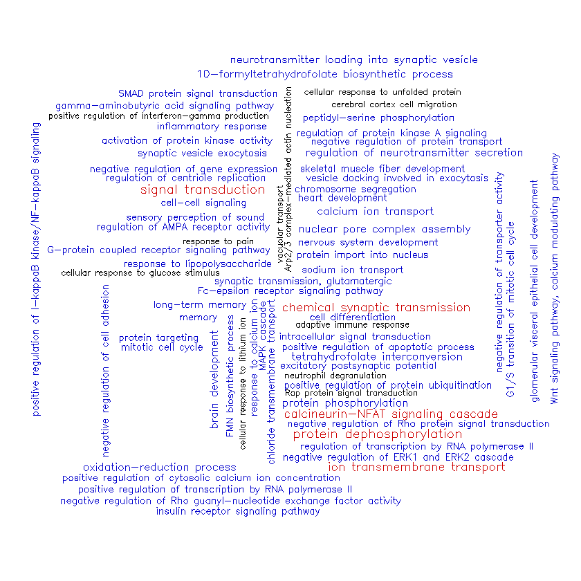
Very interesting! In contrast to the genes in cluster #1, those in cluster #2 seem to be strongly associated with communication between brain cells (“chemical synaptic transmission”, “ion transmembrane transport”, “neurotransmitter loading into synaptic vesicles”, “excitatory postsynaptic potential”, etc.) as well as intracellular signaling pathways (“signal transduction”, “protein dephosphorylation”, “calcineurin-NFAT signaling cascade”, etc.). We might have expected cluster #2’s genes to be involved in different biological processes than cluster #1 considering how well-separated they are in the space defined by the first two principal components (see plot above).

Finally, here’s cluster #3.

set.seed(412)

# ...and cluster #3
wordcloud(names(hip_terms03_table),as.numeric(hip_terms03_table),
          scale=c(1.1, .5),min.freq=2, max.words=100, random.order=T,
          rot.per=.25, colors=c('black', 'blue3', 'red3'),
          vfont=c('sans serif','plain'))

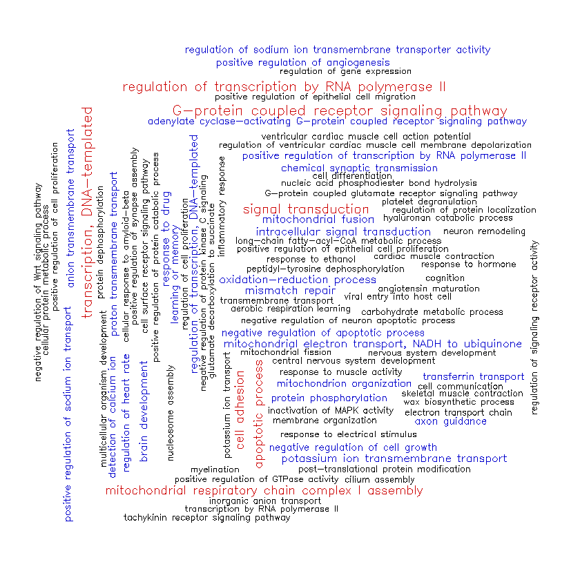
Cluster #3 looks similar to cluster #1 in some ways. It shares cluster #1’s participation in signal transduction, transcription, and cell adhesion, but includes a higher frequency of terms associated with mitochondrial structure/function (such as “mitochondrial respiratory chain complex I assembly”, “mitochondrion organization”, and “mitochondrial fusion”). Cluster #3 also has genes involved in regulating ion transport across cell membranes (“regulation of sodium ion transmembrane transporter activity”, “proton transmembrane transport”, “potassium ion transmembrane transport”, etc.).

Take-Aways

These cloud visualizations are really helpful in investigating whether the different clusters we put our dementia genes in correspond to different biological processes. While there is some overlap between the biological processes represented in all three clusters, and especially between clusters #1 and #3, each appear to have significant differences. Having some idea of these differences could help in interpreting the results of models that use the medoids of these clusters as features.

As always, thanks for reading and happy coding :)