Hi, everyone! In the last post to this blog, we talked about how to use the clValid package for R to try multiple different clustering algorithms with a range of different values for the number of clusters, \(k\), in a single function call. In this post, we go one step further and use the results of a clustering experiment to create new features to put into models.

On tap for this post:

1. Load Libraries & Data - If you’re running the Jupyter notebook version of this post from a cloned copy of the project repository on GitHub, the code blocks in this section will get you all set up.

2. \(k\)-Medoids Clustering Using CLARA - We’ll use the CLARA (Clustering Large Applications) algorithm to perform \(k\)-medoids clustering on gene expression levels for genes that were identified as being differentially-expressed in the hippocampus (a region of the brain involved in memory formation) of dementia patients. We’ll also produce some visualizations!

3. Extracting Cluster Medoids & Creating New Features - The cluster package makes it very easy to extract the medoid values for each sample.

4. Reshaping a Dataset & Adding The New Features - We’ll reshape a table consisting of pathological and other measurements taken from multiple samples from the same patients then add our new variables to it to get it in shape for model building.

Let’s do it!

Load Libraries & Data

The clara() method is available in the cluster package along with a whole slew of other clustering algorithms. CLARA is a way of doing \(k\)-medoids clustering on larger numbers of observations. We only have 277 genes that we’re trying to cluster in this example but that’s ok. CLARA will still work just fine.

library(data.table)     # I/O
library(cluster)        # CLARA clustering algorithm

Now we’ll load the data we need, which consists of:

1. A normalized table of FPKM values - These are the gene expression levels from RNA-seq experiments that have been normalized for both gene length and between-sample technical variation. Once again, this open-source data is available from the “Downloads” section of the Aging, Dementia, and TBI Study website from the Allen Institute for Brain Science.

2. Information about the samples & donors - This contains donor demographic and medical history information but, more importantly for our purposes, it has the variables that connect the brain tissue samples for which we have gene expression information to the donors they come from.

3. Brain region-specific lists of genes that appear to be differentially-expressed in samples from donors with dementia - These are the genes that we identified as having different expression patterns in dementia patients (check out this post for additional information).

4. Gene Information - This is a table of Entrez Gene identification numbers (those are the row names in our FPKM matrix), gene symbols, and gene names.

5. Gene Annotation Lists - In the last post about the project, we used the mygene package from Bioconductor to access an open-source database of even more information about genes. We generated three lists of so-called gene ontology information regarding where the gene products are active, what they do, and which biological processes they’re involved in. We’ll use these lists together with the other information about genes (from #4) to learn about the medoids we’ll use as cluster representatives.

After loading the data, we’ll make sure the gene expression data is a numeric matrix of scaled FPKM values and then subset it to contain only the hippocampus samples and the differentially expressed genes.

# load normalized FPKM values, sample info, DE gene lists for brain regions, annotations
fpkm_table <- readRDS(file='data/normalized_fpkm_matrix.Rds')
sample_info <- readRDS(file='data/sample_info.Rds')
brain_reg_sig_genes <- readRDS(file='data/brain_reg_sig_genes.Rds')
genes <- readRDS(file='data/genes.Rds')
annotations <- readRDS(file='data/hip_annotation_lists.Rds')

# make FPKM numeric matrix
fpkm_mat <- as.matrix(fpkm_table)
class(fpkm_mat) <- 'numeric'

# standardize
fpkm_standard_mat <- t(scale(t(fpkm_mat)))

# pull out individual brain region DE gene list
hip_genes <- brain_reg_sig_genes$hip_genes

# subset FPKM matrix to just HIP samples and HIP DE genes
hip_samples <- sample_info$rnaseq_profile_id[which(sample_info$structure_acronym == 'HIP')]
hip_data <- fpkm_standard_mat[hip_genes, colnames(fpkm_standard_mat) %in% hip_samples]

\(k\)-Medoids Clustering Using CLARA

\(k\)-medoids is a partitioning method much like \(k\)-means. The difference is that in \(k\)-medoids specific data points (called medoids) are representative of clusters instead of the means of the values in the cluster. A medoid is the point in a cluster with the lowest average dissimilarity with all the other members of the cluster. Because it’s based on medoids instead of means, \(k\)-medoids is considered more robust to noise than \(k\)-means.

\(k\)-medoids can be computed using an algorithm called “partitioning around medoids”, or PAM. CLARA (Clustering Large Applications) is special version of PAM that is performed on subsets. This has the advantage of speeding up computation on datasets with large numbers of observations. The optimal set of medoids are those which minimize the mean dissimilarity between every observation in the dataset and themselves. There’s a solid overview of \(k\)-medoids and PAM here, and of CLARA here if you’re interested in more background.

Because of the sampling nature of CLARA, we’ll have to specify both the number of samples (which is equivalent to the number of times PAM is performed) and the size of the samples. As with \(k\)-means, we need to pre-specify the value of \(k\), the number of clusters. The optimal value of \(k\) was determined using the clValid package we discussed in the last post. Below is a plot of the mean silhouette value, a measure of how similar an observation is to the others in its cluster, versus \(k\) generated using clValid.

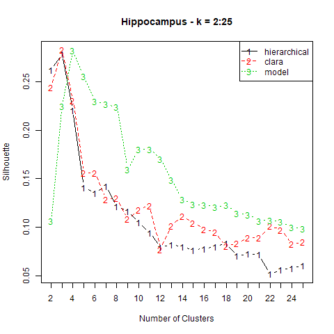
We see that the highest average silhouette value for CLARA (red) was obtained using \(k=3\). We’ll run PAM on 1000 samples of 250 observations each.

# run CLARA on HIP FPKM values
hip_final_clara <- clara(hip_data, k=3, metric = 'euclidean',
                         samples=1000, sampsize=250, pamLike=TRUE)

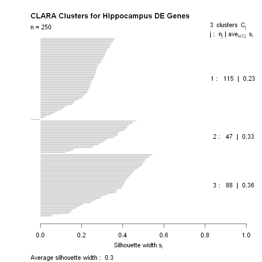
The cluster package has a plot() function in it that produces two very helpful visualizations of the resulting clustering by CLARA. The first is a principal component plot, which plots the data along the first two principal components as a way of reducing the dimensionality so the data can be visualized. The second is a plot of the average silhouette values for the observations used to determine the clustering. We’ll make the plots and discuss them in greater detail below.

plot(hip_final_clara, color=TRUE, shade=TRUE,
     labels=4, col.txt='black',
     col.p='black', col.clus=c('seagreen3', 'steelblue3', 'violetred3', 'sienna3'),
     cex=2, main = 'CLARA Clusters for Hippocampus DE Genes',
     ylim=c(-12,12),
     lwd=2,
     lty=3)

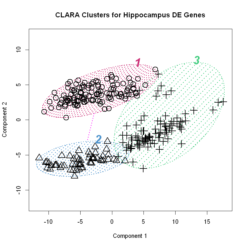
Using principal components to visualize clustering is a neat trick. Recall that principal components analysis results in a transformation of the data such that it resides in a space defined by a set of uncorrelated, orthogonal axes whereby the first direction accounts for the greatest amount of variance, the second accounts the next greatest amount, and so on. If there are natural groupings in the data, we might be able to visualize them in this new space. It’s similar to the multidimensional scaling we used on this data before. The plot() method for clara() objects draws normal confidence ellipses around the clusters to better visualize them. We can easily see in the first plot above where CLARA draws the \(k=3\) clusters we instructed it to find.

The second plot above shows how well the observations fit into their clusters. Silhouette widths range from -1 to +1 with higher values indicating that the observation has a high degree of similarity with the others in its cluster. The silhouette values in the plot above are broken up by cluster. We’re given the cluster number (\(j\)), the number of observations it has (\(n_j\)), and the clusterwise average silhouette width (\(ave_{i \in C_j}\)). We can see that only a few observations appear to be mis-clustered in cluster \(j=1\) (they’re the ones with negative silhouette widths so the bars point to the left).

Extracting Cluster Medoids & Creating New Features

With \(k\)-medoids, it’s the values of an observation that serve to represent or summarize all the members of a cluster. In the present situation, that observation is a gene, and we want to use its expression levels as a new feature for constructing models of dementia risk in patients. We have three clusters so the three medoids for those clusters will be three new features. The cluster package makes it easy to find the medoids. They’re in an attribute of the object we created when we used the clara() function. Here’s a list of everything in that object, including the medoids attribute.

names(hip_final_clara)

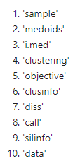
We’ll pull medoids into a variable and take a look at them for the first 10 hippocampus samples.

hip_cluster_variables <- hip_final_clara$medoids
hip_cluster_variables[ , c(1:10)]

The row names again are Entrez Gene database identification numbers. What are the names of the medoid genes? We can look in the genes table we loaded to find out!

genes[which(genes$gene_entrez_id %in% rownames(hip_cluster_variables)), ]

Where are these genes active in cells? What are they doing and what roles do they play in biological processes? We can take a look at the annotations we made last time to answer these questions. The annotations dataframe contains three lists for the three gene ontologies defined by the Gene Ontology Consortium. They are:

1. Cellular Component (CC) - This is where the gene product is found in cells or other biological structures.

2. Molecular Function (MF) - This is what the gene product does.

3. Biological Process (BP) - This is what the gene is important for.

annotations[which(rownames(annotations) %in% rownames(hip_cluster_variables)), ]

Now, this is only a partial annotation of these genes. They could have multiple entries for each ontology but when we made the lists we simplified things by only taking the most common entry for each. That having been said, the biological process ontologies for these guys fit fairly well with some of what we know about dementia and Alzheimer’s disease, namely that disrupted endocytic processes could give rise to the protein aggregation characteristic of these diseases and that adult neurogenesis in the hippocampus may be dysregulated, too\(^{1,2}\).

As much as I’d like to dig into the biology here, we’re going to push on with the data science and talk about constructing a dataset for model building.

Reshaping a Dataset & Adding The New Features

The goal of this project is to build models of dementia risk. To do that, we want our observations to be people. The problem is that we have multiple brain tissue samples from different parts of the brain for each donor. Let’s take a look at the table containing all the molecular quantifications besides gene expression levels. We download it from the study website.

# Load Luminex protein, immunohistochemistry, and isoprostane quants
neuropath_data <- data.frame(fread('http://aging.brain-map.org/api/v2/data/query.csv?criteria=model::ApiTbiDonorMetric,rma::options[num_rows$eqall]'))
dim(neuropath_data)

There are 33 variables from 377 tissue samples taken from 107 donors.

head(names(neuropath_data))

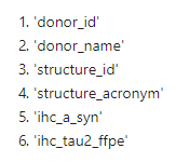
What we need is a table with donor_id down the side and each molecular measurement (such as ihc_a_syn) per brain region across the top. We’ll begin by dropping a couple of redundant variables, donor_name (not their actual name) and structure_id. We don’t need these because, essentially, the same information is in the donor_id and structure_acronym variables, respectively.

# drop donor_name and structure_id (not needed)
cols_to_remove <- c('donor_name', 'structure_id')
neuropath_data <- neuropath_data[ , !(names(neuropath_data) %in% cols_to_remove)]

That should take us down to 31 columns.

dim(neuropath_data)

We can think of this data as being in “long format” with respect to structure_acronym when we’d rather have it in “wide format” (for a good discussion of the difference, see this blog post). To get it into “wide format”, with donor_id down the side and the quantifications per brain region across the top, we can use the reshape() function. For our purposes, we’ll set the idvar argument equal to donor_id. That’s the variable we want to identify our observations by. We set timevar equal to structure_acronym since we want to have our quantification variables by brain region, or structure. We’ll take a look at the first few rows and a few random variables to see what reshape() does.

# reshape to wide format, donor_id down the side, variables by brain region across the top
reshaped <- reshape(neuropath_data, direction = 'wide',
                    idvar = 'donor_id', timevar = 'structure_acronym')
reshaped[c(1:5), c(1, 12, 37, 68, 101)]

As you can see, R has added the brain region each quantification is from to the column name. FWM, PCx, and TCx stand for “forebrain white matter”, “parietal cortex”, and “temporal cortex”, respectively. Those are the other three brain regions besides the hippocampus (HIP) in the dataset.

Now if we check the dimensions of the reshaped dataframe, we should have 107 rows (for 107 donors) and several more columns than the 31 we had before.

dim(reshaped)

Excellent! We’ll go ahead and set the row names as donor_id.

# set donor_id as row names
rownames(reshaped) <- reshaped$donor_id
reshaped$donor_id <- NULL

Now, we’re going to rename the rows and columns of the new hippocampus gene cluster variables. We’ll give the variables names in the format that R has for the rest of the variables after reshaping them, with the structure acronym after a dot following the name of the quantification. The columns we’ll label with the donor_id. Finally, we’ll transpose so that we end up with donors down the side and the new variables across the top.

# change rownames
rownames(hip_cluster_variables) <- c('gene_cluster01.HIP', 'gene_cluster02.HIP', 'gene_cluster03.HIP')

# set colnames to donor_ids corresponding to rnaseq_profile_ids (colnames for hip_cluster_variables)
colnames(hip_cluster_variables) <- sample_info$donor_id[which(sample_info$rnaseq_profile_id %in% colnames(hip_cluster_variables))]

# transpose for merging
hip_cluster_variables <- t(hip_cluster_variables)

head(hip_cluster_variables)

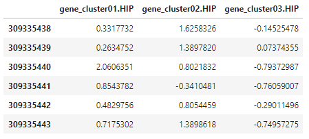
Now it’s just a matter of merging the reshaped molecular quantification dataframe with the one containing the new gene cluster variables, hip_cluster_variables. The reshaped dataframe initially had 107 rows and 116 columns after we set donor_id as the row names. After setting donor_id as the row names in the new, merged dataframe, we should still have 107 rows but now have 119 columns since we will have added the three gene cluster variables.

# add HIP genetic variables
data_plus_hip <- merge(reshaped, hip_cluster_variables, by='row.names', all=TRUE)

# clean up row names
rownames(data_plus_hip) <- data_plus_hip$Row.names
data_plus_hip$Row.names <- NULL

dim(data_plus_hip)

That looks right! We can take a peak at the new variables, which were added to the very end of the table.

data_plus_hip[c(1:5), c(114:119)]

There they are! The dataset is starting to look like something we can use for building models of dementia risk. We just need to add gene expression level cluster variables for the the remaining three brain regions (FWM, PCx, & TCx) and some additional demographic and medical history data.

Soon, we’ll talk about using the finalized dataset to build models to predict dementia risk from this data. As you might have noticed, there’s more features than samples (\(p>n\)) in our case so we’ll discuss modeling strategies that can accomodate that situation.

Thanks for reading!

References

1. Ubhi, K. & Masliah, E. (2013). Alzheimer’s Disease: Recent Advances and Future Perspectives. J Alzheimers Res. 33: S185-S194.

2. Marlatt MW, Lucassen PJ. (2010). Neurogenesis and Alzheimer’s disease: Biology and pathophysiology in mice and men. Curr Alzheimer Res. 7(2): 113-25.