Back again! I’m taking a break from thesis writing to share some of the awesome tools I’ve discovered over the course of completing this project.

In the last post, we discussed some of the results I got using hypothesis testing to identify genes differentially expressed (DE) in dementia from the Allen Institute for Brain Science’s Aging, Dementia, and TBI Study RNA-seq dataset. We identified four sets of DE genes from tissue samples from four different regions of the brain: hippocampus (HIP), forebrain white matter (FWM), parietal cortex (PCx), and temporal cortex (TCx). In the process, we significantly reduced the size of the gene expression level portion of the dataset. However, there are still 100s or 1000s of genes in each group, each of which could be considered a potential feature (or predictor) in a model of dementia risk in patients. How can we combine this data to generate a smaller set of features to use in models of dementia risk in patients?

There are several different methods for clustering data in a meaningful way. There are also several different metrics that can be used to decide on the method and parameter settings that work best on the data we have. Here, I’ll introduce the clValid package for R\(^1\). This package lets us try several different algorithms and computes a variety of metrics to compare them on, including some based on gene characteristics.

On tap for this post:

1. Clustering Methods & Validation Metrics - Brief descriptions;
2. Install Packages - We’ll install clValid and its dependent packages from CRAN and several other packages from Bioconductor for gene annotation;
3. Load Data - Load & subset a matrix of gene expression counts;
4. Generate Functional Annotation Lists - We’ll use the mygene package to access open-source gene annotation information from a maintained database (MyGene.info);
5. A Simple Clustering Optimization Experiment - A short-and-sweet example of using clValid.

Let’s get started!

Clustering Methods & Validation Metrics

Clustering Algorithms Available in clValid

The clValid method allows for the evaluation of up to eight different clustering algorithms at one time:

1. Agglomerative Hierarchical Clustering - One of - if not the - most commonly used clustering algorithms. In hierarchical clustering, all of the observations (or genes, in our case) start out in their own clusters and then are merged according to some measure of similarity (or dissimilarity).

2. K-means - Another common clustering method, K-means works iteratively to divide the data into a pre-specified number of \(k\) clusters by minimizing the within-cluster sum of squares. K-means only works with Euclidean distances (as opposed to Pearson correlation distances, for example).

3. DIANA - DIANA stands for DIvisive ANAlysis. It’s the opposite of agglomerative clustering in that, instead of each gene starting in its own cluster, all the genes start in one big cluster. The algorithm then divides that cluster up until each observation is in its own cluster.

4. PAM - AKA “Partitioning Around Medoids”. PAM, like K-means, starts with a pre-specified number of \(k\) clusters. Unlike K-means, however, PAM can accommodate distances other than Euclidean ones.

5. CLARA - CLARA is the same algorithm as PAM except that it’s implemented on subsets to speed up computation time.

6. FANNY - (Noticing a pattern here :) ) FANNY is an algorithm for fuzzy clustering where the result is not a single cluster assignment for each observation but instead a vector for each observation containing the partial membership it has in each cluster. Cluster assignments can be collapsed to a single cluster by choosing the one where the observation’s partial membership is highest.

7. SOM - This “Self-Organizing Map” algorithm utilizes artificial neural networks to produce a lower-dimensional representation of high-dimensional data. Much like the multidimensional scaling experiments discussed in earlier posts (here and interactive plots here), SOMs are terrific for visualizing complex, high-dimensional data.

8. Mixture Model-based clustering - In this method, the data is modeled as a mixture of Gaussian distributions where each distribution (or, component) represents a cluster. Expectation-maximization is used to determine the observations most likely to belong to each component.

The first five methods are implemented using functions either from base R, such as hclust() for hierarchical clustering, or from the cluster package. The SOM functions are part of the kohonen package and mixture model clustering is accomplished using the mclust package.

Validation Metrics

clValid provides three different types of validation metrics:

Internal Metrics
Internal metrics measure attributes of the clusters themselves. These are things like how well the clusters are separated from each other, or how compact they are. clValid can generate values for three such metrics:

• Connectivity - This measures how well the algorithm places observations that are close to each other in the original data space in the same cluster\(^2\). Connectivity values can range from 0 to \(\infty\) with smaller values representing “better” clustering.

• Silhouette Width - The silhouette value is a common metric for evaluating clustering experiments. It measures the confidence we have in the assignment of a given observation to a particular cluster\(^3\). The “width” is the average of these values. Like the silhouette value itself, the silhouette width can range from -1 to +1 with values closer to +1 indicating better cluster assignments.

• Dunn Index - The Dunn Index is a ratio of the shortest distance between observations not in the same cluster to the greatest distance between clusters\(^4\). Ideally, observations not in the same cluster would be far from one another so higher Dunn indices are better.

Stability Metrics
clValid can compute several metrics using something like “leave-one-out” cross-validation, where each sample is systematically excluded from the clustering experiment and the results compared with clustering on the full dataset\(^3\). Essentially, these metrics measure how well clustering results hold up when individual samples (or columns) are removed. As you might imagine, calculating these metrics can be computationally intensive if there are many samples. Nonetheless, they could be important indicators of how well a clustering strategy might handle new data. Four stability metrics are generated by clValid:

• Average Proportion of Non-Overlap (APN) - This is the average proportion of observations that end up in different clusters when samples are removed when compared to the clusters they’re in when all the samples are used. Obviously, we want this number to be small. The APN can range from 0 to 1.

• Average Distance (AD) - Similar to APN, AD is the average within-cluster distance between observations when clustered using the full dataset and with each column removed. It’s similar to connectivity in that it ranges from 0 to \(\infty\) and values close to zero are considered better.

• Average Distance between Means (ADM) - ADM looks at the average distance that observations have between themselves and the mean value (or the “center”) of the cluster they’re assigned to, and how that changes when one sample is left out. Again, ADM values closer to zero are indicators of greater stability.

• Figure of Merit (FOM) - In computing this metric, clValid measures the average error in assigning observations from the left out sample to clusters based on the remaining samples. We also want this to be close to zero.

It’s worth noting that these metrics are more easily interpretable when clustering is based on Euclidean distances versus Manhattan or Pearson correlation distances. ADM and FOM are only available for Euclidean distances.

Biological Metrics
One of the coolest things about clValid is its capacity to generate measures of how well a clustering algorithm produces results that make sense biologically. Calculating these metrics for the gene expression data we’re working with here requires us to pre-classify the genes according to one or more gene ontologies in process called functional annotation. Essentially, we tag the genes in our dataset with labels that tell us what biological processes they’re involved in, or where their products are found in the cell, so that, when we cluster them, we can see how well genes involved in the same things or found in the same places cluster together. There are two metrics we can use to evaluate this \(^3\):

• Biological Homogeneity Index (BHI) - The BHI measures how many genes in each cluster belong to the same functional category. It ranges from 0 to 1 and larger values are indicitive of more functionally homogeneous clusters.

• Biological Stability Index (BSI) - Like the other stability metrics, the BSI is calculated using a “leave-one-out” strategy. The cluster assignments for genes in similar functional classes when one sample is left out are compared to those generated using all the samples. As with the BHI, BSI ranges from 0 to 1 and larger values indicate greater stability.

We’ll discuss functional annotation in greater detail below when we actually do it!

Install Packages

Here, we’ll install clValid (and it’s dependencies) from CRAN (The Comprehensive R Archive Network) and some annotation packages from Bioconductor. The biological validation functions of clValid require the Biobase, annotate, and GO.db packages from Bioconductor and we’ll use mygene to annotate the lists of genes that are differentially-expressed in tissue samples from dementia sufferers.

IMPORTANT NOTE: If you’re trying this at home, be sure to only run this next code block once!

# install clValid and dependencies from CRAN
install.packages(c('cluster', 'kohonen', 'mclust', 'clValid'), repo='https://CRAN.R-project.org/')

# get the biocLite() installer from Bioconductor
source('https://bioconductor.org/biocLite.R')
biocLite()

#
biocLite(c('Biobase', 'annotate', 'GO.db', 'mygene'))

Now, we go ahead and load the libraries. I’m explicitly loading the two clValid dependencies we’ll use in this example, cluster and mclust, that contain the functions for the actual clustering algorithms. In this example, we won’t be using SOM so I’ve left off the kohonen package. It throws a lot of warnings at me because I have an older version of R installed. I’m including them here because there’s other information in the warnings about other dependencies that is perhaps good to know (also to show that it still works despite the warnings).

# load libraries
library(clValid)
library(cluster)
library(mclust)
library(Biobase)
library(annotate)
library(GO.db)
library(mygene)

Load Data

The next code block loads three files from a directory called data.

A Quick Aside: A Jupyter notebook version of this post is available in the project repository on GitHub. If you clone the repository, you’ll get the data folder as well as the notebook, which is located in blog-notebooks. You can run the notebook from within the cloned repo and everything should work (open source and reproducability, hooray!).

Anyways, the three files we’re loading here are:

1. A normalized matrix of FPKM values from the Allen Institute for Brain Science’s Aging, Dementia, and TBI Study. It’s a 50,283 x 377 gene-by-sample matrix of normalized gene expression counts.

2. A dataframe containing information about the brain tissue samples the gene expression data came from; for example, which region of the brain they were taken from. Today, we’re only going to be working with data from hippocampal samples.

3. Lists of the “differentially expressed in dementia” genes for each of the brain regions in the dataset (including the hippocampus).

After we load the data, we’ll convert the FPKM table to a numeric matrix and standardize it along rows (or, along genes).

# load data
fpkm_table <- readRDS(file='data/normalized_fpkm_matrix.Rds')
sample_info <- readRDS(file='data/sample_info.Rds')
brain_reg_sig_genes <- readRDS(file='data/brain_reg_sig_genes.Rds')

# make a numeric matrix
fpkm_mat <- as.matrix(fpkm_table)
class(fpkm_mat) <- 'numeric'

# standardize
fpkm_standard_mat <- t(scale(t(fpkm_mat)))

Now, we grab just the hippocampal DE genes and use the sample info to identify which samples - each of which is labeled with a unique rnaseq_profile_id - came from the hippocampus. Finally, we’ll subset our matrix of standardized FPKM values so that it only includes hippocampal DE genes and samples.

# HIP FPKM subset
hip_genes <- brain_reg_sig_genes$hip_genes
hip_samples <- sample_info$rnaseq_profile_id[which(sample_info$structure_acronym == 'HIP')]
hip_data <- fpkm_standard_mat[hip_genes, colnames(fpkm_standard_mat) %in% hip_samples]

Generate Functional Annotation Lists using mygene

At this point, we have a bunch of genes (277 to be exact) from hippocampal samples in the variable hip_data that we’d like to cluster in a meaningful way. How can we classify these genes according to their biological function so we can tell if our clustering results make sense with what we know the genes do?

Enter the mygene package! mygene is an R package that allows us to access a maintained database of gene ontology information. What’s a gene ontology (GO)? In short, it’s the gene’s function or location; what it does, where it’s product is, or what biological processes it participates in. According to the Gene Ontology Consortium, an organization dedicated to making sure we’re all on the same page in terms of information about genes, it’s “the concepts or classes used to describe gene function, and relationships between these concepts.” The Consortium’s GO Project maintains a centralized resource of information about genes. One of the ways we can use this resource is via mygene.info, which stores GO information in an easily searchable “NoSQL” database (ElasticSearch). We can access this database via the functions in the mygene package for R (there’s also a Python version).

The rows of our matrix are labeled with unique Entrez Gene database identification numbers. Using the queryMany() function from mygene, we can look up these numbers in mygene.info’s database and get GO information about each gene in our matrix. We’ll get the gene symbols, too, in case we need them.

# gene ontology info + symbols for Entrez IDs
hip_res <- queryMany(rownames(hip_data), scopes='entrezgene', fields=c('go', 'symbol'), species='human')

Let’s take a look at the first ten entries:

# take a look at the first few entries
head(hip_res, 10)

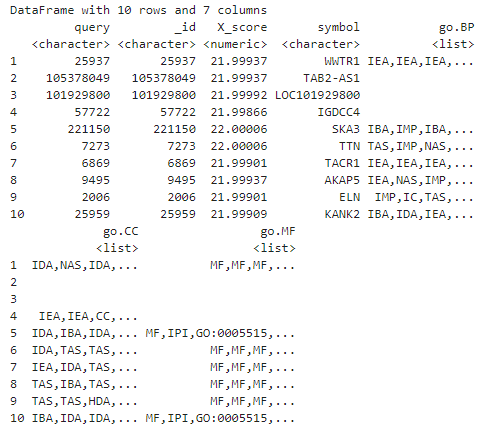
queryMany() returns a dataframe in R by default (though you can override this using the return.as argument to generate a list or text). If you’re familiar with Python, this object is a lot like a series of nested dictionaries. The GO information is contained in three “lists of lists” inside the dataframe, each corresponding to one of the three gene ontologies recognized by the Consortium:

1. Cellular Component (CC) - Generally, where the product of the gene is in a cell. Examples might be “nucleus” or “mitotic spindle”. In the dataframe above, this is in the go.CC list.

2. Molecular Function (MF) - This is what the gene product does, like “RNA binding” or “protein kinase”. It’s in go.MF.

3. Biological Process (BP) - The Consortium defines this as “pathways and larger processes made up of the activities of multiple gene products”. It would be something like “estrogen signalling” or “protein degradation”. It’s in the go.BP list from mygene.info.

In the dataframe above, we’re also given query, which is what we told it to search for (the Entrez Gene IDs). You’ll notice it’s the same as _id, the record identifier in the mygene.info database. We also have symbol (because we asked for it) and X_score which is a measure of how well mygene’s search algorithm did (we can ignore that). We’ll need the Entrez IDs later so we’ll just pull them out now (we could just as well get them from the original FPKM matrix row names).

# pull out Entrez Gene IDs
hip_entrez <- hip_res$query

Let’s take a peak at the CC GO information for the first gene, Entrez Gene 25937, or WWTR1.

# take a look at a few individual gene ontology records; CC for gene #1 (Entrez Gene #25937, WWTR1)
hip_res[1, 'go.CC'][[1]]

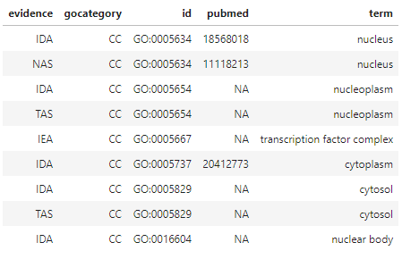
term is what we’ll eventually use to annotate our gene list for clustering validation. Some of these terms are associated with pubmed numbers linking them to peer-reviewed publications in NCBI’s PubMed database, which is nice. evidence contains standardized codes from the GO Consortium that indicate how the information in term came to be determined. “IDA”, for example, stands for “Inferred from Direct Assay”, which is pretty strong evidence that what’s in term is the truth, while “IEA” - Inferred from Electronic Annotation” - is considered weaker evidence. If we wanted to, we could filter the results to exclude terms with weaker evidence.

To make things simple, we’ll extract the most common term value for each gene and put it in a list. We’ll identify the genes with no terms by virtue of the fact that they have lists with length = 0. We’ll label their ontology as ‘unknown’. We’ll create separate lists for all three ontologies then combine them into a single dataframe.

# initialize lists
hip_cc <- NULL
hip_mf <- NULL
hip_bp <- NULL
for(i in 1:length(hip_genes)){
    # each if-else checks each 'term' list's length and, if zero, marks as 'unknown'.
    # if not zero, returns the most common function

    #### ~*~*~*~*~* Cellular Component *~*~*~*~*~ ####
    if(length(hip_res[i, 'go.CC'][[1]]$term) == 0){
        a_hip_cc <- 'unknown'
    }
    else{
        a_hip_cc <- tail(names(sort(table(hip_res[i, 'go.CC'][[1]]$term))), 1)
    }
    hip_cc <- c(hip_cc, a_hip_cc)

    #### ~*~*~*~*~* Molecular Function *~*~*~*~*~ ####
    if(length(hip_res[i, 'go.MF'][[1]]$term) == 0){
        a_hip_mf <- 'unknown'
    }
    else{
        a_hip_mf <- tail(names(sort(table(hip_res[i, 'go.MF'][[1]]$term))), 1)
    }
    hip_mf <- c(hip_mf, a_hip_mf)

    #### ~*~*~*~*~* Biological Process *~*~*~*~*~ ####
    if(length(hip_res[i, 'go.BP'][[1]]$term) == 0){
        a_hip_bp <- 'unknown'
    }
    else{
        a_hip_bp <- tail(names(sort(table(hip_res[i, 'go.BP'][[1]]$term))), 1)
    }
    hip_bp <- c(hip_bp, a_hip_bp)
}

# combine into dataframe with Entrez Gene IDs as rownames
hip_fc <- data.frame(cbind(hip_cc, hip_mf, hip_bp))
rownames(hip_fc) <- hip_entrez
colnames(hip_fc) <- c('CC', 'MF', 'BP')

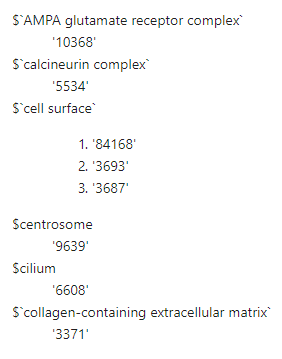
Finally, we’ll use tapply() to create a list of cellular component functional classes and the names of the hippocampal DE genes in them.

# generate a list of cellular component functional classes & the Entrez IDs in them
hip_fc_cc <- tapply(rownames(hip_data), hip_fc$CC, c)

Here’s what the final CC annotation list looks like.

head(hip_fc_cc)

An Example Clustering Optimization Experiment

Now that we have our annotation list, we’re ready to try out a few clustering algorithms on the hippocampal gene expression data. We’ll try hierarchical clustering, DIANA, and mixture models over a range of \(k=[2..6]\) clusters on a matrix of Euclidean distances. For the hierarchical clustering, we’ll use complete linkage. Finally, we’ll specify that it produce both internal and biological metrics with the latter based on the cellular component annotation list we constructed above.

To review: We’re going to construct 5 versions each of hierarchical, DIANA, and model-based clustering solutions, and compute three internal metrics and two biological ones - one of which is calculated using the “leave-one-out” strategy. We have 99 samples and 277 genes. I’m writing this on my laptop which is an old Dell XPS L421X with an Intel i7-3517U CPU. Just for curiosity, we’ll time it.

start <- Sys.time()
hip_valid <- clValid(hip_data, 2:6,
                     clMethods = c('hierarchical', 'diana', 'model'),
                     validation = c('internal', 'biological'),
                     maxitems = length(hip_genes),
                     metric = 'euclidean',
                     method = 'complete',
                     annotation = hip_fc_cc,
                     verbose = FALSE)
stop <- Sys.time()
duration <- stop-start

print(paste('Experiment duration:', round(duration, 2)))

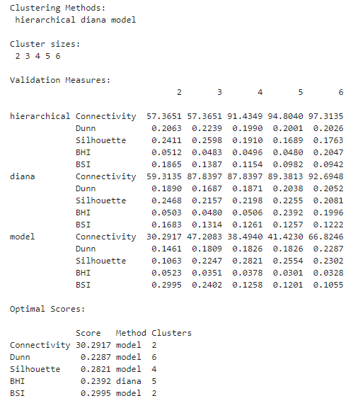
The experiment took 11 minutes. We can use summary() to take a look at the results.

summary(hip_valid)

The optimal scores can be accessed separately as well.

optimalScores(hip_valid)

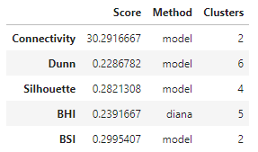
In this experiment, it looks like clustering the genes using a Gaussian mixture model resulted in the best values for 4 out of the 5 metrics calculated, albeit for different numbers of clusters. The exception is the BHI, where the DIANA solution gave the highest value.

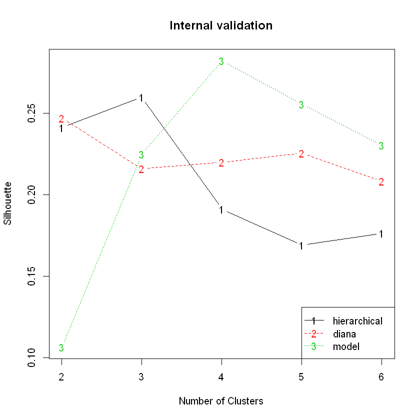
We can plot the metrics versus the number of clusters, \(k\), for each algorithm. Here’s an example using the silhouette width metric.

plot(hip_valid, measure = 'Silhouette', legendLoc = 'bottomright')

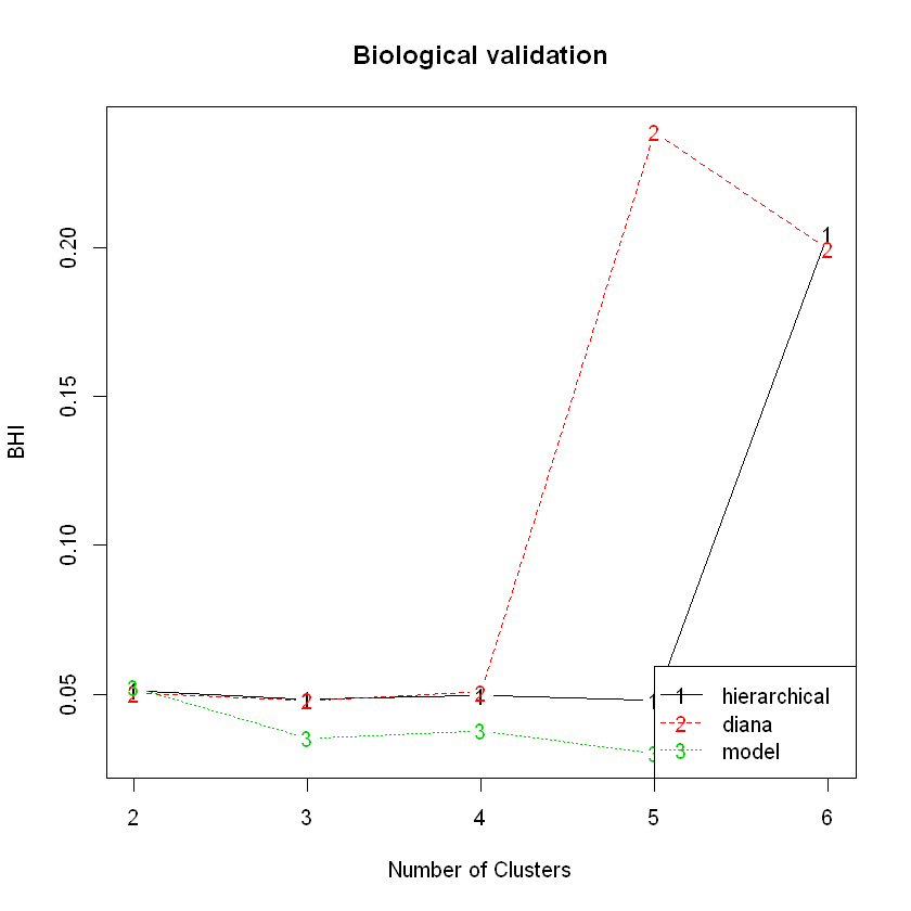
Here’s the BHI plot:

plot(hip_valid, measure = 'BHI', legendLoc = 'bottomright')

Take-Aways

clValid is a great way to try out several different clustering algorithms and values for \(k\) at one time. You can even extend this to trying different distance measures, linkage types, and/or annotation lists by calling it from within loops. The one drawback is that, depending on the number of observations, testing a wide range of \(k\) values can take a long time. I’ve looked into ways to run it in parallel on an NVIDIA GPU that could work. At least for hierarchical clustering, I could maybe replace the hclust() calls in clValid() with the gputools version, gpuHclust(). I haven’t tried it yet, though. The snow package might be a way to run clValid on a cluster of workstations. Regardless, it’s still a good way to try a bunch of different algortihms and parameters at once, which is useful considering that clustering seems to be more of an art than a science.

Happy modeling!

References

1. Brock, G., Pihur, V., Datta, S., Datta, S. (2008). clValid: An R Package for Cluster Validation. Journal of Satistical Software, 25(4).
2. Handl J., Knowles J., Kell D.B. (2005). Computational Cluster Validation in Post-Genomic Data Analysis. Bioinformatics, 21(15): 3201-12.
3. Datta S. & Datta S. (2003). Comparisons and Validation of Statistical Clustering Techniques for Microarray Gene Expression Data. Bioinformatics, 19(4): 459-66.
4. Dunn J.C. (1974). Well Separated Clusters and Fuzzy Partitions. Journal on Cybernetics, 4: 95-104.