
Hypothesis Testing for Differential Gene Expression
dementia R-stats statistics RNA-seq Now that we’ve done a little exploration of the gene expression data from the Allen Institute’s Aging, Dementia, & TBI study, we’re ready to get down to the business of identifying genes or groups of genes that could be good predictors in a model of dementia status. To do this, we’ll use hypothesis testing to determine if the expression levels for a given gene differ between Dementia and No Dementia brain tissue samples. And since we’ll be creating a family of these tests - one for each of 20,000+ genes we have - we have to talk about correcting for multiple comparisons as well.
On tap for this post…
- Preliminaries - We’ll discuss RNA-seq as a Poisson process and how the gene expression data it produces is best modeled.
- Estimating gene dispersions - We need to estimate the amount of variability there is in a gene’s expression level.
- Using Fisher’s Exact Test & correcting for multiple comparisons - This will tell us if there’s a statistically significant difference in expression level between Dementia and No Dementia samples. We’ll discuss correcting for multiple comparisons, why it’s important, and the difference between controlling for family-wise error rate and false discovery rate.
There’s a Jupyter notebook version of this post in the project repo on GitHub.
Let’s get started!
Preliminaries
High-throughput sequencing methods like RNA-seq are Poisson point processes…
RNA-seq, like other techniques that incorporate high-throughput DNA sequencing, is a Poisson point process. To see this, imagine the genome as being a long, straight line with each gene being a box along that line. We can think of these sequencing methods as randomly pointing to one of the boxes (gene \(g\), for example) and recording a count (or “hit” or “success”). Then it moves to another position along the genome (perhaps to gene \(1\)) and records a count there, and so on.
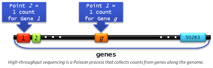
When sequencing a genome, each of our biological samples should have the same number of copies of what it is we’re sampling from for the point process. The number of “counts” (or “hits”, or “successes”) we get within a certain section of the genome (such as a gene) would be described by a Poisson distribution with some rate parameter, \(\lambda\).
…But RNA-seq data is best fit by a negative binomial distribution
With RNA-seq, we’re sampling from multiple copies of mRNA transcripts instead of a single copy of a genome. The number of transcripts for a given gene can exhibit small variations between biological replicates even when controlling for everything else. Because of this, instead of one Poisson distribution, the counts from RNA-seq are better described by a mixture of Poissons. The negative binomial distribution is frequently used to model the counts from RNA-seq because it can be interpreted as a weighted mixture of Poissons (specifically one where the \(\lambda\)s of those Poissons are gamma-distributed). In order to use hypothesis testing to determine whether or not a gene has different counts of transcripts in Dementia versus No Dementia samples, we need to estimate their variance, or dispersion (\(\phi\)).
Estimating gene dispersions
There are several different methods for estimating a gene’s dispersion that seem to vary in the amount of information used from other genes\(^1\). On one end of the spectrum, we could treat each gene independently and estimate the dispersion from its own counts alone. These estimates tend to be incorrect for a few reasons:
- There are typically only a few counts inside a given gene (AKA “successes”) but many, MANY counts outside that gene (AKA “failures”). As a result, dispersion estimates can get really big.
- A given gene’s expression level is likely to be related to those of other genes, so taking into account some of the additional information contained in the dataset can result in more accurate dispersion estimates.
Very briefly, the method we’ll use here uses a separate model to produce three types of dispersion estimates\(^2\):
- Common dispersion - This is an estimate made under the rule that all the genes must end up with the same dispersion value.
- Trended dispersion - Each gene has its own dispersion but they are smoothed according to the average counts for that gene in the dataset. This has the effect of shrinking the individual dispersions towards a shared trend.
- Tagwise dispersion - Individual dispersions that are also regularized (like trended) except towards the common dispersion calculated of a subset of neighboring genes.
The function below imports a subset of the gene expression data from samples from the same brain region (hippocampus, forebrain white matter, parietal cortex, temporal cortex) or donor sex group (male, female; see the project repo on GitHub for more details). After some tidying up, the counts are filtered and normalized before estimates are made for the common, trended, and tagwise dispersions. The output is saved to an .Rds file as well as returned.
library(edgeR)
prep_count_mat <- function(group, filter_counts, filter_samples, ...){
    # 1. get file & tidy it up
    x_counts_status <- data.frame(read.csv(paste('data/', group, '_counts_status.csv', sep='')))
    rownames(x_counts_status) <- x_counts_status$X
    x_counts_status$X <- NULL
    colnames(x_counts_status) <- substring(colnames(x_counts_status), 2)
    # 2. Extract status row and delete from count mat; make counts numeric
    x_status <- unlist(x_counts_status[50284,])
    x_counts <- as.matrix(x_counts_status[1:50283,])
    class(x_counts) <- 'numeric'
    x_counts <- round(x_counts)
    # 3. Make DGEList object
    x_dgeList <- DGEList(x_counts, group = x_status)
    # 4. Filter to exclude with fewer than 'filter_counts' number of counts in 'filter_sample' number of samples
    x_filtered <- x_dgeList[rowSums(1e+06*x_dgeList$counts/expandAsMatrix(x_dgeList$samples$lib.size, dim(x_counts))>filter_counts)>=filter_samples,]
    print(paste('Number of genes left after filtering: ', dim(x_filtered)[1]))
    # 5. Normalize
    x_norm <- calcNormFactors(x_filtered)
    # 6. Estimate common dispersion
    x_norm <- estimateGLMCommonDisp(x_norm, verbose = TRUE)
    # 7. Estimate trended dispersion
    x_norm <- estimateGLMTrendedDisp(x_norm)
    # 8. Estimate tagwise ("gene-wise") dispersions
    x_norm <- estimateGLMTagwiseDisp(x_norm)
    # save object to .Rds file
    saveRDS(x_norm,file=paste('data/',group,'_norm_counts_disp.Rds',sep=''))
    # also return it for hypothesis tests below
    return(x_norm)
}
For demo purposes, we’ll use the data from parietal cortex (‘pcx’) tissue samples.
pcx_norm <- prep_count_mat('pcx',2,10)
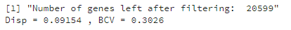
The function prints the output of estimateGLMCommonDisp() which includes the common dispersion (‘Disp’) and the biological coefficient of variation (BCV). BCV is equal to the square root of the common dispersion.
round(sqrt(pcx_norm$common.dispersion), 4)

It is interpreted as the relative variability of the real expression levels (as opposed to the estimates we make from the data)\(^2\). A BCV of 0.3026 is saying that, if we could accurately measure the expression levels in our samples, we would see that they vary when compared to each other by about \(\pm30\%\) on average.
Fisher’s Exact Test & correcting for multiple comparisons
The problem with multiple comparisons
To test for differences in the counts for a given gene between groups, we’ll use Fisher’s Exact Test. exactTest() is the edgeR version that we’ll use here. For this test, the null hypothesis is that there is no difference in the counts in Dementia and No Dementia samples.
Fisher’s Exact Test is so-called because the p-value can be calculated exactly, as opposed to being estimated. Unfortunately, there’s a problem when running multiple hypothesis tests that arises directly from the definition of a p-value; namely, that it is the probability of rejecting the null hypothesis by mistake when it’s actually true. A p-value of 0.05 means that there is a 5% chance that we could be rejecting the null hypothesis by mistake and thus creating a false positive result. If we ran 100 such tests, each with a significance level (\(\alpha\)) of 0.05, we’d expect to have ~5 false positives simply by chance.
As the number of tests increases, so does the number of potential false positives. In our case, we have 20,599 genes. If we test each at the \(\alpha=0.05\) level, we could have as many as \(20599 \times 0.05 = 1030\) genes that we’d say are differentially expressed between Dementia and No Dementia samples but really aren’t.
Correcting for multiple comparisons: family-wise error rate (FWER) vs. false discovery rate (FDR)
The effect of multiple comparisons is to make the p-values we get from the exact tests unreliable for deciding whether to reject the null hypothesis. One common method of overcoming this, is to divide the \(\alpha\) value by the number of tests performed and use that value as the new cutoff for rejection. In the context of a multiple comparisons problem, \(\alpha\) is the family-wise error rate (FWER) and dividing it by the number of tests is known as the Bonferroni correction.
The FWER is the probability of at least one incorrect rejection of the null hypothesis in our family of tests. Because of this, controlling the FWER using the Bonferroni correction is a stringent procedure, resulting in very few false positives. This comes at the cost of more false negatives, though, and that can be a problem when there are 20,000+ tests. For \(\alpha = 0.05\), the Bonferroni correction would have us reject the null hypothesis when \(p < 0.05 \div 20599 = 0.00000244\). Not many genes are going to have differences in the number of counts big enough to result in a p-value that small. We’re likely to fail to reject null hypotheses when we should.
A more powerful means of correcting for multiple comparisons is to control the false discovery rate (FDR). The FDR is the proportion of rejected null hypotheses that are mistakes. By controlling for the proportion of mistakes rather than the probability of at least one of them, controlling the FDR is a less stringent procedure, resulting in more false positives than the Bonferroni correction but substantially fewer false negatives (and therefore greater statistical power).
There are different methods to control the FDR. The one we’ll use here is called the Benjamini-Hochberg (BH) procedure\(^3\). After running the exact tests, the function below uses topTags() to perform the BH adjustment and saves the top 1000 genes sorted by the uncorrected p-value. We’ll return the uncorrected results of exactTest().
# function to perform Fisher's Exact Test/p-value correction & save results
# Takes arguments:
#   1. norm_counts = output from prep_count_mat function above
#   2. group = hip, fwm, pcx, tcx, male, or female
#   3. disp = common, trended, tagwise, or auto (auto picks the most complex dispersion available)

test_genes <- function(norm_counts, group, disp, ...){
    # perform Fisher's Exact Test
    x_test <- exactTest(norm_counts, pair = c('No Dementia' , 'Dementia'), dispersion = disp)
    # BH adjustment
    x_table <- topTags(x_test, n = 1000, adjust.method = 'BH', sort.by = 'PValue')
    saveRDS(x_table, file=paste('data/',group,'_exact_test_results_',disp,'.Rds',sep=''))
    return(x_test)
}
Let’s run the tests for the parietal cortex data. In the following, p.value is an argument for topTags() and refers to the adjusted p-value. Choosing auto selects the “most complex” dispersion in the object, which in our case is the tagwise one.
pcx_results <- test_genes(pcx_norm, 'pcx', 'auto', p.value = 0.05)
One thing we can do with the output of exactTest() is to classify genes into three groups based on the corrected p-value and the \(log_2\) fold-change between groups:
- Significant and upregulated
- Not significant, or
- Significant and downregulated versus No Dementia samples.
To do this, we use decideTestsDGE() with BH as the correction method and 0.01 as the adjusted p-value cutoff for rejecting the null hypothesis.
summary(decideTestsDGE(pcx_results, adjust.method = 'BH', p.value = 0.01))
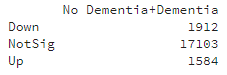
That’s 3496 genes that are differentially expressed in samples of the parietal cortex from Dementia donors versus those from No Dementia donors.
Conclusions & Next Steps
My primary goal in this post was to work through some of the statistics under the hood of differential expression analysis. I’m anxious to take a closer look at the results. In the next post, I hope to have some interesting visualizations to show you and some genes to tell you about.
Until then, thanks for reading and happy coding!
References
-
Landau WM & Liu P. (2013). Dispersion estimation and its effect on test performance in RNA-seq data analysis: a simulation-based comparison of methods. PLOS ONE. 8(12): e81415.
-
McCarthy DJ, Chen Y, & Smyth GK. (2012). Differential expression analysis of multifactor RNA-seq experiments with respect to biological variation. Nucleic Acids Research. 40: 4288–97.
-
Benjamini, Y, & Hochberg, Y. (1995). Controlling the false discovery rate: a practical and powerful approach to multiple testing. Journal of the Royal Statistical Society B. 57: 289-300.